1. Text Dataset (RedPajama)
RedPajama is a large open-source pre-training corpus stored in Parquet format. For this benchmark a representative subset is loaded across three epochs, varying batch sizes to study the effects of shuffling strategy and data-loading mechanics on overall training throughput.
1.1 Top-level Results
Across all batch sizes, Ray Data (lazy random_shuffle) consistently shows:
- Longest elapsed training time
- Lowest samples/sec feeding rate
- Highest data-stall percentage
- Highest RAM usage (~3 GB vs ~1 GB for WebDataset and MDS)
- Lowest GPU utilization
The root cause is Ray's lazy global random shuffle, which is triggered at first batch iteration. At that point Ray spawns reader workers, writes Arrow tables to its shared Object Store, adds a random float column to each row, then performs a distributed range-based sort-merge across all partitions.
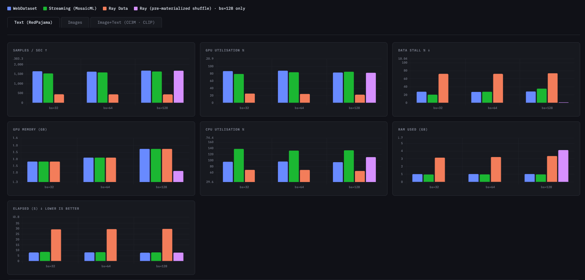
AVG across 3 epochs · WebDataset (blue) · Streaming/MosaicML (green) · Ray Data (orange) · Ray pre-materialized (purple, bs=128 only)
1.2 How Ray's Global Shuffle Works
ds = ray.data.read_parquet("parquet_path")
  .random_shuffle()   # lazy — deferred until first iteration
  .materialize()      # forces eager execution into Object Store
Step 1 — Read & tag: Each reader worker reads assigned shards into PyArrow tables and appends a random float shuffle key to every row, writing results to the Ray Object Store.
Reader Worker 0:  shards 0,1  →  ObjStore partition A
Reader Worker 1:  shards 2,3  →  ObjStore partition B
Step 2 — Distributed Sort-Merge: Reducer tasks perform a range-based sort across all partitions, collecting rows by key range and merge-sorting within each range, then writing final shuffled partitions back.
Rows with key [0.0, 0.5)  →  Reducer 0  →  output_partition_0
Rows with key [0.5, 1.0]  →  Reducer 1  →  output_partition_1
Memory Note: PyArrow tables are immutable. Every sort pass requires a full allocation of new memory for the sorted result. A ~700 MB raw dataset can consume ~3 GB of RAM during shuffle — roughly 4–5× raw size.
1.3 Effect of Pre-Materialization
To isolate the shuffle cost from batch serving, a separate run using .materialize() before iteration was conducted at batch_size=128. With pre-materialization:
- Ray's sample feeding rate and total training time drop to match WebDataset and MDS levels
- GPU utilization recovers
- Data-stall percentage falls sharply
This confirms the bottleneck is the lazy shuffle, not Ray's serving pipeline itself.
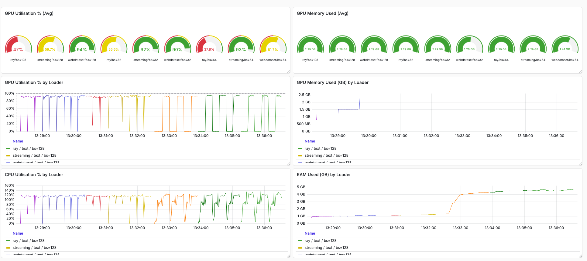
Grafana dashboard: GPU utilization gauges (top), time-series GPU utilization, GPU memory, CPU utilization, and RAM used per loader across the full training run.
1.4 Recommended Ray Usage Pattern
For production training loops with Ray Data, load once into the Object Store and shuffle per-epoch:
ds = ray.data.read_parquet(path).materialize()  # load once, cache in Object Store

for epoch in range(num_epochs):
    # Lightweight: reorders block references only (no data copy)
    epoch_ds = ds.randomize_block_order()

    # Alternatively, for stronger shuffle:
    # epoch_ds = ds.random_shuffle().materialize()

    for batch in epoch_ds.iter_batches(batch_size=128):
        ...  # training step
1.5 Shuffling Comparison
| Attribute | WebDataset .shuffle(1000) | MosaicML MDS py1s | Ray Data random_shuffle |
|---|---|---|---|
| What is shuffled? | Sample bytes in sliding buffer | Global index array (integers) | Sample bytes in Object Store |
| Shuffle scope | Window of 1000 samples | Global (true 1/N) | Global (true 1/N) |
| Memory for shuffle | ~50 MB buffer | ~200 KB index only | 1 GB+ Object Store |
| First-batch latency | Same as subsequent | Same as subsequent | Much higher (sort-merge delay) |
| Random I/O required? | No (sequential .tar reads) | Yes (.mds seek by index) | No (sequential after materialise) |
| Shuffle quality | Poor (local window) | Excellent | Excellent |
| Best storage type | HDD / S3 / spinning disk | NVMe / SSD | Any (sequential read after mat.) |
| Multi-node scaling | Shard-level only | Node-local global | True distributed global |