LLM Data Pipeline Benchmark Report
A Deep Dive into WebDataset · MosaicML Streaming · Ray Data
April 2025 · Workloads: Text · Image · Multimodal (CC3M)
This report benchmarks three PyTorch-compatible data loading libraries across text, image, and multimodal workloads. Metrics collected include total training time, sample feeding rate (samples/sec), data stall percentage, RAM usage, GPU utilization, and CPU utilization. Each loader was evaluated at multiple batch sizes over three epochs.
Libraries Under Test
| Library | Format | Primary Strength |
|---|---|---|
| WebDataset | .tar shards | Sequential streaming, decode offload |
| MosaicML StreamingDataset | .mds binary | True global shuffle, NVMe-optimized |
| Ray Data | Parquet | Distributed multi-node training |
Key Findings
Finding 1 — Ray Data shuffle overhead
Ray's random_shuffle() is lazy: it triggers a sort-merge over Arrow tables in shared Object Store memory on first iteration, pushing RAM to ~3 GB for a 700 MB dataset and causing severe first-batch latency spikes.
Finding 2 — Pre-materializing Ray resolves the bottleneck
Using .random_shuffle().materialize() before iteration brings Ray's throughput and GPU utilization in line with the other two loaders.
Finding 3 — WebDataset decode offload delivers 2× GPU utilization
WebDataset's built-in .decode() offloads JPEG decoding to worker subprocesses via Pillow C bindings, delivering roughly 2× higher GPU utilization and ~50% lower training time versus in-process decoding.
Finding 4 — MosaicML MDS py1s: true global shuffle at ~200 KB The py1s shuffle achieves true global shuffle quality with only ~200 KB of index memory (vs 1 GB+ for Ray), at the cost of random I/O — well-suited to NVMe, less so to HDD or object storage.
Dataset: Text (RedPajama) · Images · Image+Text (CC3M) · GPT-2 / ResNet-18 / CLIP · Tesla V100
LLM Data Pipeline Benchmark
AVG across 3 epochs · 3 loaders × 3 datasets × 3 batch sizes
| Metric | wds-32 | wds-64 | wds-128 | str-32 | str-64 | str-128 | ray-32 | ray-64 | ray-128 | ray-pms-128 |
|---|---|---|---|---|---|---|---|---|---|---|
| samples/sec | 1,649.6 | 1,628.1 | 1,683.5 | 1,536.4 | 1,588.6 | 1,637.4 | 450.0 | 446.6 | 444.0 | 1,678.1 |
| GPU util % | 87.0 | 88.1 | 83.1 | 79.1 | 83.9 | 85.3 | 25.4 | 24.4 | 22.5 | 82.4 |
| GPU mem GB | 2.82 | 3.11 | 3.75 | 2.82 | 3.11 | 3.75 | 2.82 | 3.11 | 3.75 | 2.13 |
| CPU util % | 96.0 | 96.8 | 94.7 | 138.2 | 132.6 | 133.6 | 69.4 | 69.2 | 65.8 | 111.2 |
| RAM used GB | 1.02 | 1.03 | 1.03 | 0.97 | 0.98 | 0.98 | 3.15 | 3.23 | 3.36 | 4.13 |
| Data stall % | 27.8 | 27.3 | 28.4 | 20.5 | 27.7 | 35.5 | 72.5 | 72.5 | 73.8 | 1.32 |
| Elapsed s | 8.0 | 8.1 | 7.8 | 8.6 | 8.3 | 8.1 | 29.4 | 29.6 | 29.8 | 7.87 |
w=2 workers · bs=32/64/128 · avg across 3 epochs · 100k images · parallel decode in DataLoader workers vs Ray object store
| Metric | wds-32 | wds-64 | wds-128 | str-32 | str-64 | str-128 | ray-32 | ray-64 | ray-128 |
|---|---|---|---|---|---|---|---|---|---|
| samples/sec | 631.62 | 726.42 | 922.12 | 937.21 | 1018.54 | 1084.05 | 793.29 | 896.38 | 1136.59 |
| GPU util % | 20.30 | 21.95 | 25.62 | 30.42 | 31.67 | 32.44 | 23.45 | 26.07 | 34.82 |
| GPU mem GB | 0.950 | 1.174 | 1.623 | 0.950 | 1.174 | 1.623 | 0.950 | 1.174 | 1.623 |
| CPU util % | 1677.02 | 1259.67 | 1035.64 | 116.93 | 115.51 | 112.60 | 1631.70 | 1502.58 | 1283.17 |
| RAM used GB | 1.082 | 1.137 | 1.200 | 1.143 | 1.203 | 1.370 | 2.293 | 2.374 | 2.642 |
| Data stall % | 52.61 | 51.50 | 55.74 | 1.45 | 0.81 | 0.64 | 14.12 | 21.42 | 31.10 |
| Elapsed s | 158.33 | 137.78 | 108.45 | 106.73 | 98.17 | 92.34 | 126.25 | 111.70 | 88.03 |
| /dev/shm avg GB | 0.010 | 0.020 | 0.040 | 0.002 | 0.004 | 0.008 | 1.030 | 1.020 | 1.100 |
| /dev/shm peak GB | 0.019 | 0.039 | 0.077 | 0.010 | 0.010 | 0.019 | 1.163 | 1.163 | 1.297 |
| Metric | wds-32 | wds-64 | wds-128 | str-32 | str-64 | str-128 | ray-32 | ray-64 | ray-128 |
|---|---|---|---|---|---|---|---|---|---|
| samples/sec | 22.99 | 31.01 | 37.38 | 22.60 | 31.26 | 38.30 | 22.70 | 31.18 | 37.47 |
| GPU util % | 3.6 | 3.12 | 4.62 | 3.4 | 3.58 | 4.56 | 3.56 | 3.58 | 4.46 |
| GPU mem GB | 3.09 | 3.22 | 3.49 | 3.09 | 3.22 | 3.49 | 3.09 | 3.22 | 3.50 |
| CPU util % | 674.4 | 908.0 | 1104.1 | 670.4 | 921.8 | 1101.1 | 616.3 | 834.6 | 998.4 |
| RAM used GB | 7.29 | 4.37 | 2.98 | 7.31 | 4.34 | 2.88 | 9.39 | 6.48 | 5.00 |
| Data stall % | 0.65 | 0.86 | 1.04 | 0.44 | 0.73 | 0.91 | 3.71 | 5.20 | 6.43 |
| Elapsed s | 434.9 | 322.7 | 267.5 | 444.7 | 321.4 | 260.7 | 440.6 | 320.8 | 266.8 |
1. Text Dataset (RedPajama)
RedPajama is a large open-source pre-training corpus stored in Parquet format. For this benchmark a representative subset is loaded across three epochs, varying batch sizes to study the effects of shuffling strategy and data-loading mechanics on overall training throughput.
1.1 Top-level Results
Across all batch sizes, Ray Data (lazy random_shuffle) consistently shows:
- Longest elapsed training time
- Lowest samples/sec feeding rate
- Highest data-stall percentage
- Highest RAM usage (~3 GB vs ~1 GB for WebDataset and MDS)
- Lowest GPU utilization
The root cause is Ray's lazy global random shuffle, which is triggered at first batch iteration. At that point Ray spawns reader workers, writes Arrow tables to its shared Object Store, adds a random float column to each row, then performs a distributed range-based sort-merge across all partitions.
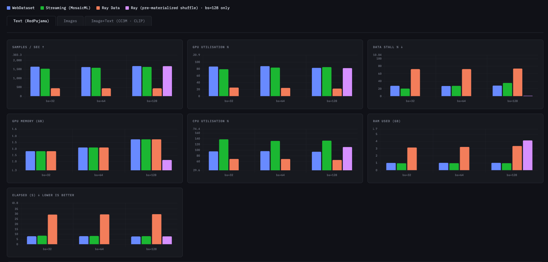
AVG across 3 epochs · WebDataset (blue) · Streaming/MosaicML (green) · Ray Data (orange) · Ray pre-materialized (purple, bs=128 only)
1.2 How Ray's Global Shuffle Works
ds = ray.data.read_parquet("parquet_path")
  .random_shuffle()   # lazy — deferred until first iteration
  .materialize()      # forces eager execution into Object Store
Step 1 — Read & tag: Each reader worker reads assigned shards into PyArrow tables and appends a random float shuffle key to every row, writing results to the Ray Object Store.
Reader Worker 0:  shards 0,1  →  ObjStore partition A
Reader Worker 1:  shards 2,3  →  ObjStore partition B
Step 2 — Distributed Sort-Merge: Reducer tasks perform a range-based sort across all partitions, collecting rows by key range and merge-sorting within each range, then writing final shuffled partitions back.
Rows with key [0.0, 0.5)  →  Reducer 0  →  output_partition_0
Rows with key [0.5, 1.0]  →  Reducer 1  →  output_partition_1
Memory Note: PyArrow tables are immutable. Every sort pass requires a full allocation of new memory for the sorted result. A ~700 MB raw dataset can consume ~3 GB of RAM during shuffle — roughly 4–5× raw size.
1.3 Effect of Pre-Materialization
To isolate the shuffle cost from batch serving, a separate run using .materialize() before iteration was conducted at batch_size=128. With pre-materialization:
- Ray's sample feeding rate and total training time drop to match WebDataset and MDS levels
- GPU utilization recovers
- Data-stall percentage falls sharply
This confirms the bottleneck is the lazy shuffle, not Ray's serving pipeline itself.
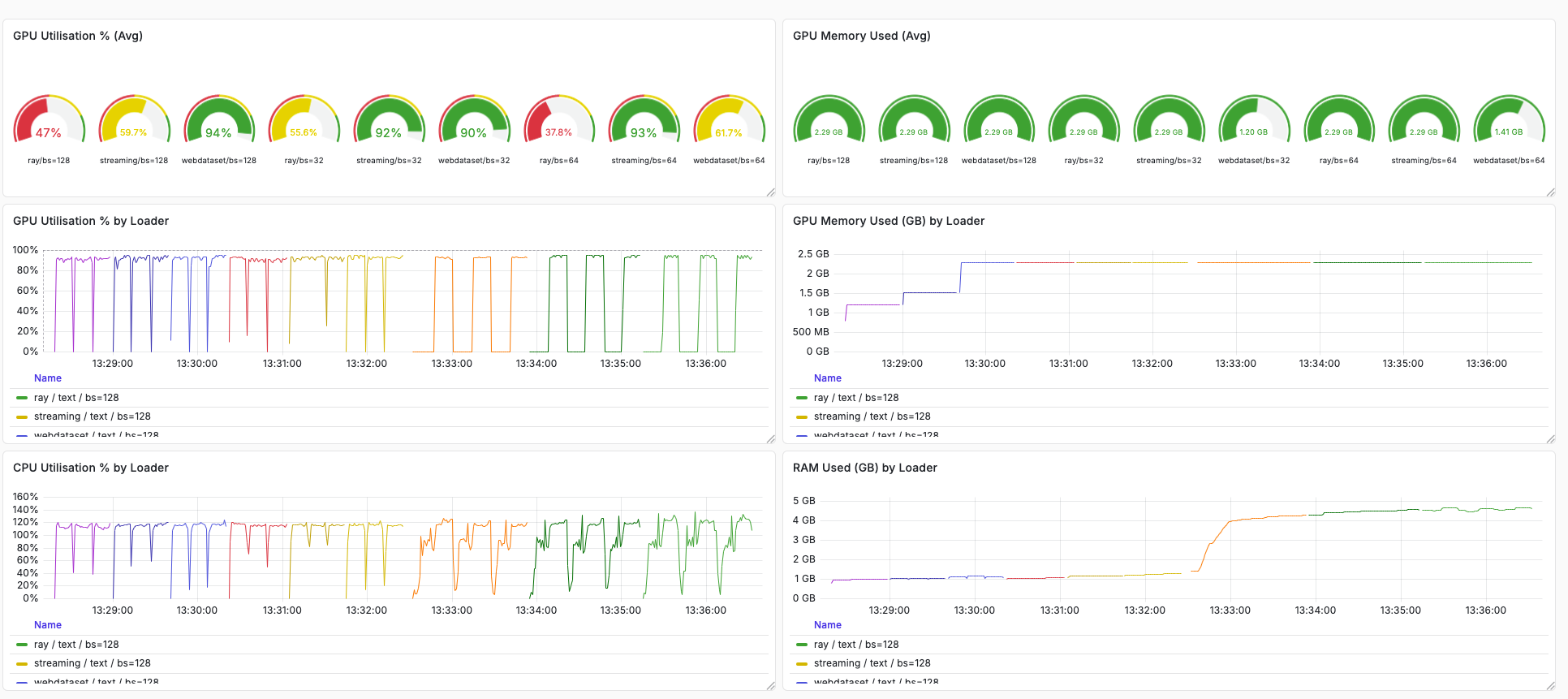
Grafana dashboard: GPU utilization gauges (top), time-series GPU utilization, GPU memory, CPU utilization, and RAM used per loader across the full training run.
1.4 Recommended Ray Usage Pattern
For production training loops with Ray Data, load once into the Object Store and shuffle per-epoch:
ds = ray.data.read_parquet(path).materialize()  # load once, cache in Object Store

for epoch in range(num_epochs):
    # Lightweight: reorders block references only (no data copy)
    epoch_ds = ds.randomize_block_order()

    # Alternatively, for stronger shuffle:
    # epoch_ds = ds.random_shuffle().materialize()

    for batch in epoch_ds.iter_batches(batch_size=128):
        ...  # training step
1.5 Shuffling Comparison
| Attribute | WebDataset .shuffle(1000) | MosaicML MDS py1s | Ray Data random_shuffle |
|---|---|---|---|
| What is shuffled? | Sample bytes in sliding buffer | Global index array (integers) | Sample bytes in Object Store |
| Shuffle scope | Window of 1000 samples | Global (true 1/N) | Global (true 1/N) |
| Memory for shuffle | ~50 MB buffer | ~200 KB index only | 1 GB+ Object Store |
| First-batch latency | Same as subsequent | Same as subsequent | Much higher (sort-merge delay) |
| Random I/O required? | No (sequential .tar reads) | Yes (.mds seek by index) | No (sequential after materialise) |
| Shuffle quality | Poor (local window) | Excellent | Excellent |
| Best storage type | HDD / S3 / spinning disk | NVMe / SSD | Any (sequential read after mat.) |
| Multi-node scaling | Shard-level only | Node-local global | True distributed global |
2. Image Dataset
The image benchmark uses a 64×64 image dataset. A key variable is where JPEG decoding happens — inside the dataloader's worker processes or in the main training process. A ResNet model is used as the training target, which requires images to be resized from 64×64 to 224×224 before ingestion.
2.1 Multi-worker/node image processing with WebDataset
Spawning worker processes with wds.WebLoader
To run image processing in parallel, wds.WebLoader spawns worker subprocesses :
wds.WebLoader(ds, batch_size=None, num_workers=num_workers, pin_memory=False,
multiprocessing_context='spawn' if num_workers>0 else None))
# NOTE that mp_ctx = 'spawn' is necessary as without this, the usual subprocess spawn method fork() after CUDA init corrupts worker CUDA context will lead to workers hang, and hence the main process won't be getting any results from the result queue, entire program hangs.
# 'spawn' starts fresh interpreter processes, avoiding inherited CUDA state.
Each worker gets a forked copy of the full pipeline and independently drives the entire chain — shard reading, shuffling, decoding, resizing, and batching — before placing the completed batch into a result queue for the main process to consume:
Worker Process (forked copy of pipeline):
    open tar shard
        ↓
    .shuffle(500)            ← runs in worker
        ↓
    .decode('rgb8')          ← runs in worker  ✓ JPEG → numpy [H, W, 3]
        ↓
    .map(_wds_decode_sample) ← runs in worker  ✓ resize → [3, 224, 224]
        ↓
    .to_tuple("jpg")         ← runs in worker
        ↓
    .batched(64)             ← runs in worker
        ↓
    puts completed batch into result queue
                ↓
Main process:  queue.get() → train(batch)
Note:
num_workersmust not exceed the number of shards — WebDataset assigns shards to workers round-robin, and any worker that receives no shard will raise aValueError.
Step1 .shuffle() — local buffer shuffle
Explained in text dataset.
Step2 .decode() — worker subprocess decodes via Pillow C lib:
WebDataset exposes a .decode() API that runs image decoding inside worker subprocesses, leveraging Pillow's C bindings.
ds = (
    wds.WebDataset(shards, shardshuffle=True)
    .shuffle(500)
    .decode('rgb8')       # decodes to numpy uint8 [H, W, 3]
    .to_tuple('jpg')
    .batched(batch_size, partial=True)
)
... if there are other processing in the pipeline for each worker, and finally the generated batch got fed into result queue for main process to consume for training.
2.2 Process images with Ray Data Operator: Transformation (map)
Ray Data exposes transformations as operators. Each operator call (.map(), .random_shuffle(), .join(), etc.) registers a step in the pipeline in the order it is called. Nothing executes until data is consumed — e.g. via iter_batches().
ds = ray.data.read_parquet(...)
ds = ds.random_shuffle()
ds = ds.map(decode_row)

for batch in ds.iter_batches(batch_size=64):  # ← triggers execution
    train(batch)
Execution order once iter_batches() is called
Step 1 — Load into object store
ray.data.read_parquet(<path>, parallelism=num_workers)
Ray reads Parquet row groups from disk in parallel and deserializes them into Arrow Tables stored in /dev/shm (the Plasma object store). The parallelism parameter controls how many blocks the dataset is split into — this also sets the granularity for all downstream operators.
e.g. 100k rows with
parallelism=50→ 50 blocks × 2,000 rows/block. Each block becomes the unit of work for.map().
Step 2 — random_shuffle() — barrier
random_shuffle() is a barrier: it waits for all blocks to land in the object store before redistributing rows across new blocks. After shuffle, the data remains split into the same number of blocks in /dev/shm, with Ray holding an ObjectRef for each.
⚠️ Pipeline order matters: if
.map()runs beforerandom_shuffle(), the shuffle barrier forces all decoded blocks (much larger) to materialise in/dev/shmsimultaneously → object store memory explosion.
Step 3 — .map() — streaming
.map() is not a barrier. With num_workers=2, Ray assigns one block per worker and streams results:
Block 0 (2k rows) → Worker 1 decodes all 2k → output block in /dev/shm
Block 1 (2k rows) → Worker 2 decodes all 2k → output block in /dev/shm
                                                        ↓
                                          iter_batches slices Block 0:
                                          batch 0: rows 0–63    → train
                                          batch 1: rows 64–127  → train
                                          ...
                                          batch 31: rows 1984–1999 → train
                                          Block 0 fully consumed → FREED from /dev/shm
                                                        ↓
Block 2 → Worker 1 (now free)             iter_batches moves to Block 1
Block 3 → Worker 2 (now free)             ...
Workers prefetch the next block while the current one is being consumed, so at most 2–3 decoded blocks live in /dev/shm at any time.
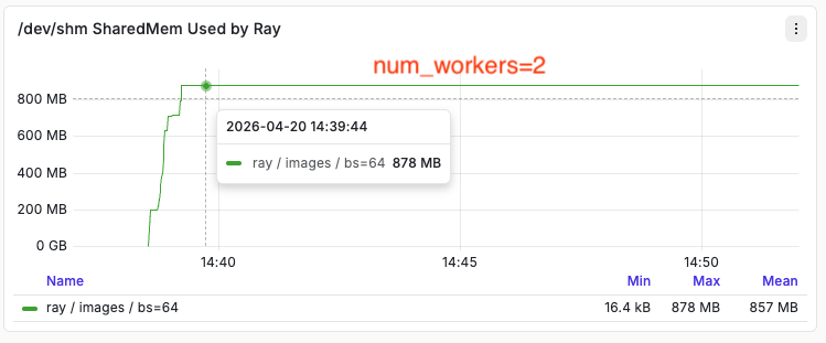
Peak /dev/shm overhead estimate (2k rows, 224×224 RGB):
3 blocks × 2,000 rows × (3 × 224 × 224 × 1 byte) = ~903 MB
Actual /dev/shm usage during the run (ray/images/bs=64/workers=2)
Key takeaways
- Pipeline order matters — always shuffle before decode.
random_shuffle()is a barrier that materialises everything before it; if that includes decoded images, object store memory explodes. parallelism(block count) matters — block size directly controls peak/dev/shmoverhead. Fewer, larger blocks = less scheduling overhead but more memory per block in flight. More, smaller blocks = finer-grained parallelism but higher orchestration cost.
2.3 Process Images with MosaicML StreamingDataset
With mds dataset, it's quite easy to do parallel image process. We just need to add additional logic after when each worker seek to the position of the sample index and read the data from disk to process the image. Decoding(or additional processing) is simply triggered per sample inside __getitem__ of the StreamingDataset (a map-style object representation), which DataLoader calls inside each worker process when num_workers > 0.
How it works
class _StreamingDecodeDataset:
    def __getitem__(self, idx: int) -> dict:
        sample = self._ds[idx]          # seek to sample by byte offset in .mds shard
        raw = sample["jpeg_bytes"]      # raw JPEG bytes
        sample["jpeg_bytes"] = _decode_resize_bytes(raw)  # decode + resize in worker
        return sample
The standard PyTorch DataLoader drives the parallelism:
DataLoader(ds, batch_size=batch_size, num_workers=num_workers,
           pin_memory=True, drop_last=True)
Worker Process 1:                    Worker Process 2:
  __getitem__(idx_0)                   __getitem__(idx_1)
    → seek shard by byte offset          → seek shard by byte offset
    → read raw JPEG bytes                → read raw JPEG bytes
    → PIL decode + resize 224×224        → PIL decode + resize 224×224
    → return dict                        → return dict
          ↓                                    ↓
          └──────────── result queue ──────────┘
                              ↓
          Main process: collate → batch [B, 3, 224, 224] → train
Key differences from WebDataset
| WebDataset | StreamingDataset | |
|---|---|---|
| Dataset style | Iterable (__iter__) | Map-style (__getitem__) |
| Shuffle | .shuffle(buffer) — approximate, in-pipeline | shuffle_algo="py1s" — epoch-level global shuffle |
| Shard access | Sequential tar scan | Random byte-offset seek per sample |
| Worker splitting | Shard-level (each worker owns shards) | Sample-level (DataLoader assigns individual indices) |
Why sample-level access is possible
MosaicML's .mds format stores a per-shard offset table that maps each sample index to its exact byte position on disk. __getitem__(idx) can seek directly to any sample without scanning. This is what makes random sample access efficient and enables per-sample DataLoader worker assignment.
3. Multimodal Dataset (CC3M)
The multimodal benchmark uses a 10,000-sample subset of the Conceptual Captions 3M (CC3M) dataset, storing image+caption pairs in each of the three formats. CC3M contains variable-resolution images, which creates an important constraint: WebDataset's default collate_fn cannot batch tensors of different spatial dimensions.
3.1 Variable-Resolution Constraint
Unlike the fixed 64×64 images in the image benchmark, CC3M images span a wide range of resolutions. WebDataset's .decode() produces numpy arrays whose H×W varies per sample; batching these into a single tensor requires all samples in a batch to have identical shape.
Consequence: For the multimodal benchmark, .decode() is disabled for WebDataset. All three loaders deliver raw image bytes to the main training loop, which performs per-sample decoding and resizing before collation.
This levels the playing field across all three loaders: the primary performance differentiator shifts from loader-level decode efficiency to sequential per-sample preprocessing throughput.
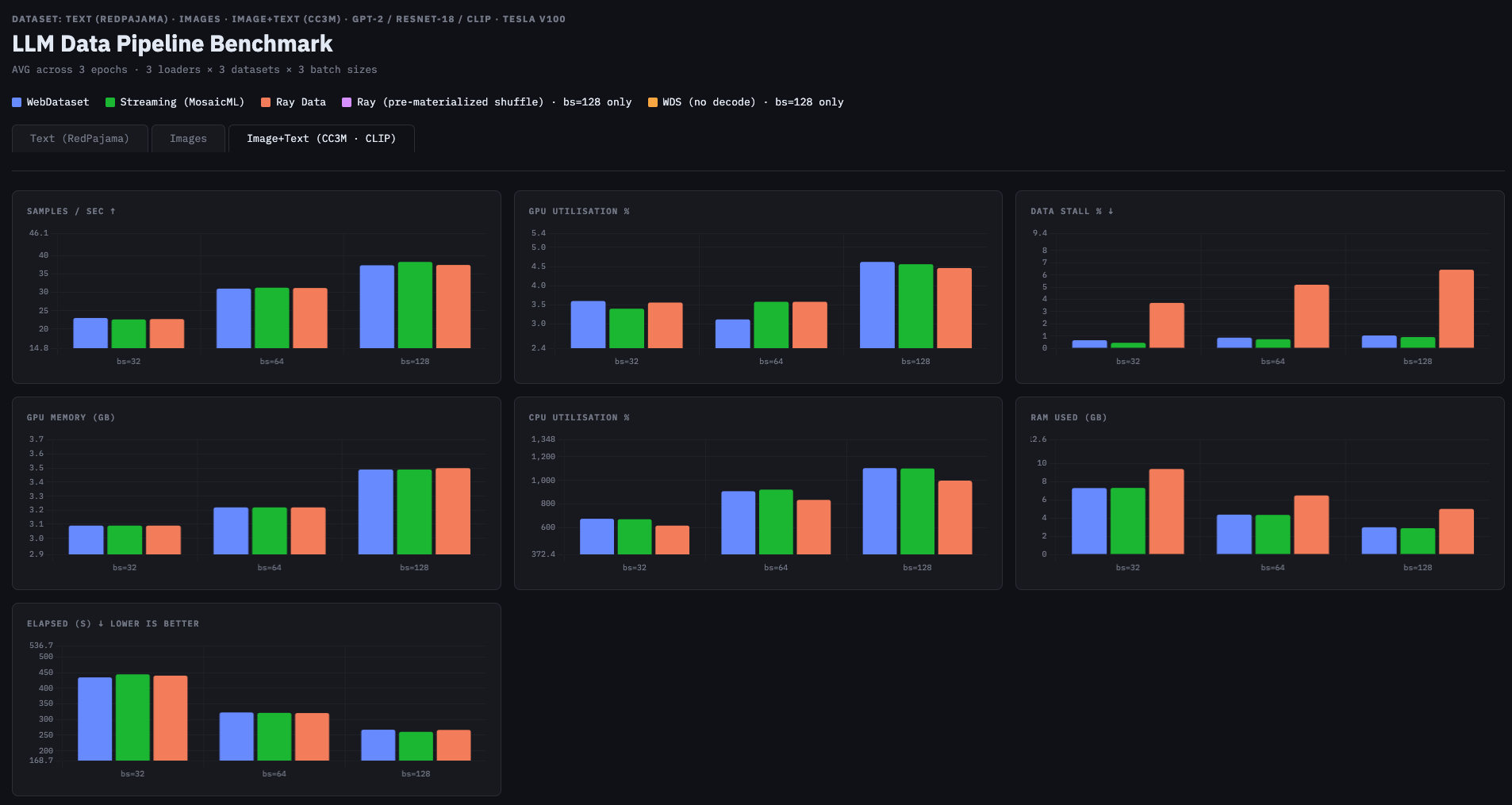
Image+Text (CC3M · CLIP) results. All three loaders operate on raw bytes passthrough — decode offload is disabled due to variable-resolution images. Performance differences reflect sequential preprocessing throughput.
3.2 Format Comparison for Multimodal Storage
| Aspect | WebDataset (.tar) | MosaicML MDS | Ray Data (Parquet) |
|---|---|---|---|
| Access pattern | Sequential only | Random access (O(1) seek) | Sequential (Parquet rowgroup) |
| Multimodal support | Native (key-matched files in .tar) | Native (arbitrary fields per sample) | Requires separate image col (bytes) |
| Decode offload | Yes (.decode() API) | No built-in decode hook | No built-in decode hook |
| Variable-size images | Yes (bytes passthrough) | Yes (bytes passthrough) | Yes (bytes passthrough) |
| Shuffle quality | Buffer (window-limited) | Global (py1s) | Global (sort-merge) |
| Shard format | .tar (sequential) | .mds (binary, indexed) | .parquet (columnar) |
4. Recommendations & Decision Guide
4.1 When to Use Each Loader
| Scenario | Recommended Loader | Rationale |
|---|---|---|
| Streaming from S3 / HDD / slow NFS | WebDataset | Sequential .tar reads; no random I/O penalty |
| High-quality shuffle on NVMe / SSD | MosaicML MDS (py1s) | True global shuffle at near-zero memory cost; optimal for fast random read storage |
| Multi-node distributed training | Ray Data | Native distributed shuffle and execution model across cluster nodes |
| Image/video workloads needing decode offload | WebDataset | .decode() offloads to worker C libs; clearest GPU utilization gains |
| Pre-tokenized text, large batch sizes | MosaicML MDS or WebDataset | Both show lower memory and stall overhead than lazy Ray shuffle |
| Multimodal with variable-resolution images | Any (with bytes passthrough) | Disable loader-level decode; manual resize + collate required for all loaders |
4.2 Shuffle Strategy Quick Reference
WebDataset
Use shardshuffle=True + .shuffle(N) for cheap local randomization; acceptable for most NLP pre-training where perfect shuffle quality is not critical.
MosaicML MDS py1s Best for single-node NVMe workloads; delivers true global shuffle with negligible memory overhead; degrades on HDD due to random seek pattern.
Ray Data random_shuffle
Use .materialize() before epoch iteration to avoid first-batch latency spike; consider .randomize_block_order() for cheaper inter-epoch reshuffling.
4.3 Memory Footprint Summary
| Loader | Shuffle Memory Overhead | Notes |
|---|---|---|
| WebDataset | ~50 MB (buffer) | Buffer size controlled by .shuffle(N) |
| MosaicML MDS (py1s) | ~200 KB (index array) | Only integer indices stored; sample bytes not loaded until accessed |
Ray Data (random_shuffle) | 1 GB+ (Object Store) | Arrow table immutability forces double-allocation during sort-merge; scales with dataset size |
| Ray Data (pre-materialised) | Same 1 GB+ | Materialization pays the cost upfront; subsequent epochs cheaper with randomize_block_order() |
Appendix — MDS Format & py1s Shuffle Deep Dive
A.1 MDS Shard Structure
When prepare_dataset.py runs MDSWriter, it produces the following layout (5,000 samples/shard by default):
mds/
  index.json           ←  manifest: shard sizes, per-sample byte offsets
  shard.00000.mds      ←  samples 0 – 4,999
  shard.00001.mds      ←  samples 5,000 – 9,999
  shard.00002.mds      ←  samples 10,000 – 14,999
  ...
# Each .mds shard is a flat binary file:
#   [sample_0_bytes] [sample_1_bytes] ... [sample_4999_bytes]
#   with a front-of-file index for O(1) random access by position
Key Difference from WebDataset:
.tarfiles require sequential reads from the start of the archive..mdsfiles expose an index for O(1) seek to any sample by global position — enabling efficient random-access patterns like py1s.
A.2 py1s Shuffle Mechanics
py1s = Python implementation · single-pass · shuffle
Algorithm:
- Read
index.jsonto obtain global sample indices[0, 1, 2, ..., N-1] - Shuffle the index array in-place:
[23401, 7832, 41205, 891, ..., 15634] - Partition the shuffled index evenly across
num_workersDataLoader workers - Each worker uses its index slice to seek into
.mdsshards and read sample bytes on demand
# py1s worker assignment example (num_workers=4, N=50,000)
Worker 0 indices: [23401, 7832,  41205, 891,  ...]  # 12,500 samples
Worker 1 indices: [33201, 19832,  5205, 2891, ...]  # 12,500 samples
Worker 2 indices: [43401, 27832, 31205, 1891, ...]  # 12,500 samples
Worker 3 indices: [13401, 37832, 11205, 4891, ...]  # 12,500 samples

# Worker 0 resolves index 23401:
# → shard 4  (23401 // 5000 = 4)
# → position 3401 within shard.00004.mds
# → O(1) seek → read sample bytes → decode
Why memory is only ~200 KB: The shuffle operates entirely on the integer index array — no sample bytes are moved or copied. Only when a worker needs a specific sample does it seek and read from disk.