Distributed ML Notes
Engineering notes on distributed ML systems — written from an infrastructure perspective. The focus is on the system design problems underneath the ML abstractions: data movement at scale, distributed compute coordination, memory hierarchies, and the operational failure modes that textbooks skip.
Content keep updating...
live site at : https://lucyge2022.github.io/Distributed-ML-Notes/index.html
Contents
Concepts
Background knowledge that cuts across all chapters.
- GPU, VRAM, PCIe & NVLink — hardware mental model: why GPUs, what VRAM is, PCIe bottleneck, NVLink
- PyTorch Memory Management — how PyTorch allocates and caches CUDA memory
Chapter 2 — Data Ingestion Patterns
How raw data gets from disk into a training loop.
- Dataset — dataset composition, IDX binary format, tensor representation, data ingestion flow
- Batching, Sharding & Caching — Ray+Parquet vs WebDataset vs MosaicML MDS: formats, sharding strategies, shuffle, remote streaming
Chapter 3 — Distributed Training Patterns
How training is parallelized across multiple machines.
- Parameter Server Pattern — PS + workers architecture, gradient flow, staleness, fault tolerance
- Worker-Only (AllReduce) Pattern — Ring AllReduce, PyTorch DDP, fault tolerance, failure analysis
Chapter 4 — Feature Store
How features are computed, stored, and served consistently between training and inference.
- Feature Store — offline vs online paths, train-serve skew, Chronon consistency measurement; illustrated with a user–restaurant recommendation system
Supplemental Code
Runnable toy programs that accompany these notes: distributed-ml-examples
| Example | What it covers |
|---|---|
| ddp-testrun | PyTorch DDP training with Ring AllReduce on MNIST |
Built with
mdBook — the src/SUMMARY.md defines the book structure.
mdbook serve   # local preview at http://localhost:3000
mdbook build   # build static site to book/
Chapter 2: Dataset
1. Dataset Composition
A dataset is split into two parts:
| Split | Purpose |
|---|---|
| Training set | Model learns from these — weights are updated based on this data |
| Test set (verification set) | Verify how well the model learned — never seen during training |
Using MNIST as example: https://www.kaggle.com/datasets/hojjatk/mnist-dataset/data
total 107344
drwxr-xr-x  3 root  staff        96 Mar 17 13:58 t10k-images-idx3-ubyte
-rw-r--r--  1 root  staff   7840016 Mar 17 13:58 t10k-images.idx3-ubyte
drwxr-xr-x  3 root  staff        96 Mar 17 13:58 t10k-labels-idx1-ubyte
-rw-r--r--  1 root  staff     10008 Mar 17 13:58 t10k-labels.idx1-ubyte
drwxr-xr-x  3 root  staff        96 Mar 17 13:58 train-images-idx3-ubyte
-rw-r--r--  1 root  staff  47040016 Mar 17 13:58 train-images.idx3-ubyte
drwxr-xr-x  3 root  staff        96 Mar 17 13:58 train-labels-idx1-ubyte
-rw-r--r--  1 root  staff     60008 Mar 17 13:58 train-labels.idx1-ubyte

train-images.idx3-ubyte  ← TRAINING images (47MB)
train-labels.idx1-ubyte  ← TRAINING labels (60KB)

t10k-images.idx3-ubyte   ← TEST images (7.8MB)
t10k-labels.idx1-ubyte   ← TEST labels (10KB)
t10k= "test 10,000" — 10,000 test images
| Count | Share | |
|---|---|---|
| Training | 60,000 | 85% |
| Test | 10,000 | 15% |
| Total | 70,000 |
2. Binary File Format (IDX)
These files use IDX format — a simple binary format invented for MNIST.
Images file (train-images.idx3-ubyte)
File size: 47,040,016 bytes

HEADER (16 bytes):
  bytes 0-3:   magic number  = 2051    (means "this is images")
  bytes 4-7:   num images    = 60,000
  bytes 8-11:  num rows      = 28
  bytes 12-15: num cols      = 28

DATA (after header):
  60,000 × 28 × 28 = 47,040,000 bytes
  47,040,000 + 16 header = 47,040,016 ✓ matches file size!
Each byte = one pixel:
0= black255= white- values in between = grey shades
This is why Parquet (or other unstructured datalake format) can be used to house unstructured datasets like images and video — it stores raw bytes per row just as well as structured columns.
Labels file (train-labels.idx1-ubyte)
File size: 60,008 bytes

HEADER (8 bytes):
  bytes 0-3:  magic number = 2049  (means "this is labels")
  bytes 4-7:  num labels   = 60,000

DATA:
  60,000 × 1 byte = 60,000 bytes
  60,000 + 8 header = 60,008 ✓ matches file size!
Each byte = one label value:
| Value | Class |
|---|---|
| 0 | T-shirt/top |
| 1 | Trouser |
| 2 | Pullover |
| ... | ... |
| 9 | Ankle boot |
3. Tensor Representation
When loaded into an ML framework, raw bytes become tensors:
- Images tensor — shape
(60000, 28, 28): 60,000 images, each 28×28 pixels, each pixel a value 0–255 - Labels tensor — shape
(60000,): a flat list of 60,000 label values
tensor([9, 0, 0, 3, 0, 2, 7, 2, 5, 5, 0, 9, ...])
         ↑ each value is the class label for that image
4. Data Ingestion Flow
Refer to load_dataset_sample_flow_explained.py for showing a simple breakdown of dataset loading process.
Binary file (on SSD)
    ↓ read bytes
In-memory array (NumPy)
  shape: (60000, 28, 28)  dtype: uint8
    ↓ convert + normalize
tf.Tensor / torch.Tensor
  shape: (60000, 28, 28)  dtype: float32
  divide by 255 → values become 0.0 to 1.0
    ↓ batch
Mini-batch tensor
  shape: (32, 28, 28)  ← 32 images at a time
    ↓ flatten for simple model
  shape: (32, 784)     ← 28×28 = 784 pixels per image
    ↓ feed into model
Forward pass!
Raw format → CPU RAM → GPU VRAM → Forward pass
Why normalize (divide by 255)? These values flow through matrix multiplications. If they stay at 0–255, gradients explode. Keeping them at 0.0–1.0 keeps the math stable.
Labels are only used during loss calculation — not fed into the forward pass.
Optional: Data Ingestion via GDS (GPU Direct Storage)
Raw format → GPU VRAM → Forward pass
With NVIDIA GDS support (cuFile API), data can be loaded directly from NVMe storage into GPU VRAM, bypassing CPU RAM entirely — eliminates a full copy in the pipeline.
[TODO] add link to ddp-testrun for dataset breakdown + feeding example
5. NumPy vs Pure Python
NumPy is a Python library for fast mathematical operations on arrays and matrices.
| Pure Python | NumPy | |
|---|---|---|
| Execution | Interpreted line by line | Written in C under the hood |
| Loops | Slow, not optimized for math | Operates on entire arrays at once |
| CPU instructions | General | Uses SIMD instructions |
| Parallelism | None | Same concept as GPU parallelism, but on CPU |
6. Why NumPy → Tensor (not just NumPy)?
Most important: NumPy has no autograd. It doesn't remember intermediate computation results, so it cannot do backprop.
A Tensor remembers every operation applied to it (the computation graph), which is what makes gradient computation possible.
Raw format → NumPy (CPU RAM) → Tensor (GPU VRAM) → Forward pass
                ↑                     ↑
         fast math, C-backed    autograd-capable, runs on GPU
Chapter 2: Batching, Sharding & Caching
Reference implementation: prepare_dataset.py
Are dataset formats framework-agnostic?
Yes — the stored format and the consuming framework are separate concerns.
The files on disk (.parquet, .tar, .mds) are just files. What ties them to a framework is the loader library you use to read them. Model-specific preprocessing (tokenization, image augmentation, feature engineering) is applied at load time as a transform/map step — it is never baked into the stored format. The same .parquet files could in principle be read by Ray, Spark, pandas, or DuckDB.
Stored format (files on disk)
        ↓  loader library reads + streams
Batches in memory (raw samples)
        ↓  transform / map function applied
Model-ready tensors (tokenized, normalized, etc.)
        ↓
Training loop
Comparison at a Glance
| Ray Dataset | WebDataset | MosaicML (MDS) | |
|---|---|---|---|
| File format | .parquet | .tar shards | .mds shards + index.json |
| Sharding unit | Row count (configurable) | Sample count per tar | Byte size limit |
| Batching direction | Horizontal (rows) | Sequential within shard | Horizontal, with random access |
| Random access | Yes (columnar index) | No (sequential only) | Yes (offset index per shard) |
| Remote streaming | Yes (S3, GCS, HDFS) | Yes (S3, GCS, HTTP, local) | Yes (S3, GCS, Azure, local) |
| Shuffle | Distributed shuffle, sort-based | Shuffle buffer (in-memory window) | Epoch-consistent, multiple algos |
| Primary consumer | Ray Train / Ray Data | PyTorch DataLoader | PyTorch DataLoader |
| Resume from checkpoint | Via Ray lineage | Manual (shard position) | Built-in (tracks seen samples) |
1. Ray Dataset + Parquet
Format
Parquet is a columnar binary format:
- Stores data column-by-column rather than row-by-row
- Built-in compression (Snappy, Gzip, Zstd)
- Schema-enforced — every file knows its column names and types
- Supports predicate pushdown — you can filter and project columns before reading any data into memory
shard-00000-of-00004.parquet
shard-00001-of-00004.parquet
...
Each shard is an independent Parquet file. Ray points at the whole directory.
Sharding pattern
Sharding is horizontal — by row count:
Full dataset: 200,000 rows
  ↓ split into 4 shards of 50,000 rows each
shard-00000: rows 0–49,999
shard-00001: rows 50,000–99,999
...
Vertical selection (loading only specific columns) is also possible via column projection — Parquet's columnar layout means unused columns are never read from disk.
Consuming with Ray
import ray

ds = ray.data.read_parquet("/path/to/parquet/")
# __id__ column present for shuffle tracking

# apply preprocessing as a map (lazy — not executed yet)
ds = ds.map(lambda row: tokenize(row["text"]))

# batch for training
for batch in ds.iter_torch_batches(batch_size=32):
    ...
Features
- Lazy materialization —
read_parquet()doesn't load data; it builds a logical plan. Data only moves when you iterate. - Parallel I/O — Ray reads multiple shards across workers simultaneously, overlapping I/O with compute
- Prefetching —
prefetch_batches=Nkeeps N batches ready ahead of the training loop - Built-in caching —
.materialize()pins a dataset in Ray object store memory so it's not re-read from disk on each epoch - Distributed shuffle — Ray can globally shuffle across all shards using a sort-based algorithm; no single-node bottleneck
2. WebDataset + .tar Shards
Format
WebDataset packs samples into standard .tar archives. Each sample is a group of files sharing a key prefix:
shard-000000.tar
  └── 000000/000000.txt    ← text content of sample 0
  └── 000000/000000.json   ← metadata of sample 0
  └── 000000/000001.txt    ← sample 1
  └── 000000/000001.json
  ...
The .tar format is universal — any tool that reads tar files can inspect the data. There is no custom binary encoding; samples are just files inside an archive.
Sharding pattern
Sharding is by sample count — write N samples per tar, then start a new one:
SHARD_SIZE = 5_000  # samples per shard

shard-000000.tar  ← samples 0–4,999
shard-000001.tar  ← samples 5,000–9,999
...
There is no random access within a shard — reading is sequential. To shuffle, WebDataset uses a shuffle buffer: load K samples into memory, pick one at random, replace it with the next sample from the stream.
.shuffle(1000) # keep 1000 samples in buffer, randomly pop from it
Consuming with PyTorch
import webdataset as wds

dataset = (
    wds.WebDataset("data/webdataset/shard-{000000..000004}.tar")
    .shuffle(1000)               # in-memory shuffle buffer
    .decode()                    # decode bytes to Python types
    .to_tuple("__key__", "txt", "json")
    .map(lambda key, txt, meta: tokenize(txt))  # model-specific preprocessing
)

loader = DataLoader(dataset, batch_size=32, num_workers=4)
WebDataset implements PyTorch's IterableDataset — it plugs directly into DataLoader.
Features
- Remote streaming — can read directly from
s3://,gs://, or HTTP URLs without downloading first; shards are fetched on demand - No local storage required — useful when dataset is larger than local disk
- Simple format —
.taris readable by any OS tool; no special library needed to inspect raw files - Multi-worker friendly — each DataLoader worker takes a different shard, no coordination needed
- Limitation — no random access, no epoch-consistent shuffle; shuffle quality depends on buffer size
3. MosaicML StreamingDataset + .mds Shards
Format
MDS is a custom binary format designed specifically for large-scale ML streaming:
mds/
  index.json          ← manifest: shard list, column schemas, sample counts
  shard.00000.mds     ← binary shard file
  shard.00001.mds
  ...
Each .mds shard has an internal offset table — a lookup that maps sample index → byte offset within the file. This enables true random access within a shard, unlike .tar which must be read sequentially.
Sharding pattern
Sharding is byte-size based — MDSWriter keeps writing rows until the shard hits size_limit bytes, then starts a new shard:
# from prepare_dataset.py:
MDSWriter(out=str(out), columns=columns, size_limit=shard_size * 2048)
# size_limit = 5000 samples × 2048 bytes ≈ 10MB per shard → 111 shards for ~1.1GB
This means shards have roughly equal byte sizes but potentially different sample counts (longer texts → fewer samples per shard).
Consuming with PyTorch
from streaming import StreamingDataset
from torch.utils.data import DataLoader

dataset = StreamingDataset(
    local="data/mds",           # local cache dir
    remote="s3://my-bucket/mds", # optional: stream from remote
    shuffle=True,
    shuffle_algo="py1s",         # epoch-consistent shuffle algorithm
)

loader = DataLoader(dataset, batch_size=32, num_workers=4)
Shuffle algorithms
MDS ships multiple shuffle algorithms as a first-class feature — unlike WebDataset where shuffle is an afterthought:
| Algorithm | Tradeoff |
|---|---|
py1s | Downloads 1 shard at a time, low memory, weaker shuffle |
py2s | Downloads 2 shards at a time, better shuffle |
naive | Full in-memory shuffle, best quality, high memory |
Features
- Random access — offset index allows seeking to any sample without reading the whole shard; enables proper epoch-consistent shuffling
- Download cache management — automatically downloads shards from remote storage to local cache as needed; LRU eviction when cache is full
- Epoch-consistent shuffle — every epoch sees all samples exactly once, in a different order; no duplicates or skips
- Resume from checkpoint — tracks exactly which samples were consumed; training can resume mid-epoch after a crash
- Schema-enforced —
index.jsonrecords column names and types; reader validates on load - Tightly integrated with LLM training stacks — used in production at MosaicML/Databricks for training models like MPT
Choosing Between Them
| If you… | Use |
|---|---|
| Already use Ray for orchestration / distributed training | Ray + Parquet |
| Have a giant unstructured dataset (images, audio, video, text) and want simplest format | WebDataset |
| Need epoch-consistent shuffle, checkpoint resume, and remote streaming for LLM training | MosaicML MDS |
| Need to run SQL-style queries or column projections on the dataset | Parquet (only columnar format) |
| Want zero infrastructure — just read from S3 with no local disk | WebDataset (lowest overhead) |
Chapter 4: ML training/serving Lifecycle - User Restaurant Recommendation example
Example system throughout this chapter: User–Restaurant Recommendation — predict P(order) for each candidate restaurant shown to a user.
Overall Platform Architecture
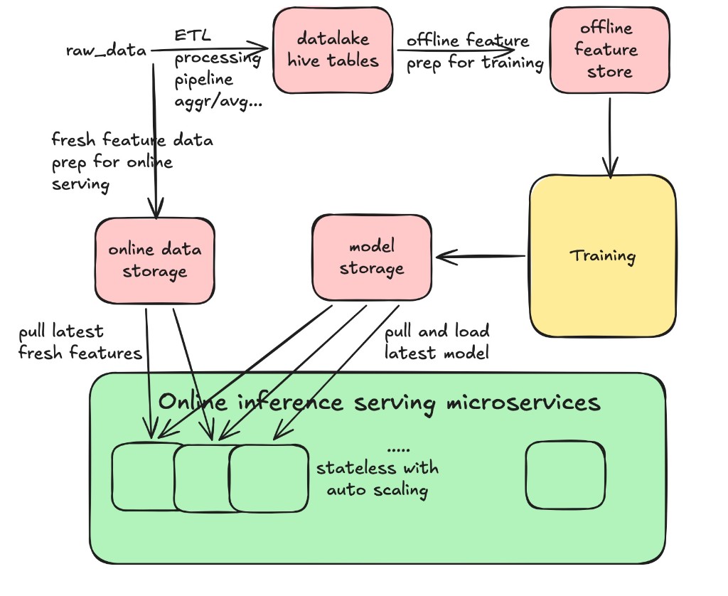
The platform has two distinct pipelines sharing the same feature definitions:
- Offline path — raw data → ETL → data lake (Hive tables) → offline feature store → training
- Online path — online data storage (fresh features) + trained model → inference serving microservices
The inference layer is stateless with auto-scaling — each serving pod pulls the latest features from online storage and the latest model from model storage independently.
The Data: Three Tables, Three Update Cadences
| Table | Key | Contents | Update frequency |
|---|---|---|---|
user_features | user_id | avg order value, food preferences, ... | Weekly |
restaurant_features | rest_id | location, food type tags, ... | Hourly |
events | (user_id, rest_id) | every impression shown, ordered=0/1 | Every impression |
The events table is the spine. It records every (user, restaurant) pair that was actually shown to a user, with ordered=1 if the user placed an order and ordered=0 if not. This is the label.
Training Cycle (Offline)
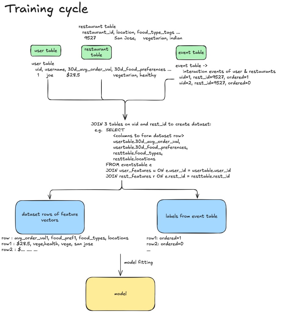
Step 1 — JOIN three tables on shared keys
The events table drives the join. For every event row, pull the matching user features and restaurant features:
SELECT
    usertable.30d_avg_order_val,
    usertable.30d_food_preferences,
    resttable.food_types,
    resttable.location,
    eventstable.ordered          -- label
FROM eventstable e
JOIN user_features u  ON e.user_id  = usertable.user_id
JOIN rest_features r  ON e.rest_id  = resttable.rest_id
Step 2 — Output two artifacts
dataset rows of feature vectors          labels from event table
────────────────────────────             ──────────────────────
row1: $28.5, vege/health, vege, SJ       row1: ordered=1
row2: $...   ...          ...  ...       row2: ordered=0
...                                      ...
The IDs (user_id, rest_id) are dropped after the join — the model trains on pure numeric feature vectors, not on identifiers.
Step 3 — Model fitting
The model learns to map:
[avg_order_val, food_preferences, food_types, location, ...] → P(order)
The trained artifact is stored in a model registry (model storage).
Inferencing Cycle (Online, e.g. target < 50ms)
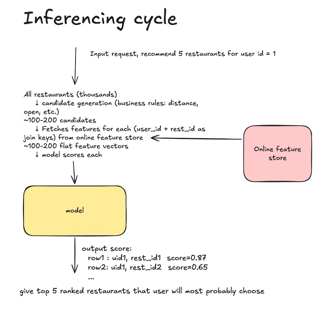
Step 1 — Candidate generation
Input: "recommend 5 restaurants for user_id = 1"
  ↓
All restaurants (thousands)
  ↓  business rules: distance, open now, cuisine filters
~100–200 candidates
This is a coarse filter using cheap rules — no model yet.
Step 2 — Feature fetch from online FeatureStore
For each of the ~100–200 candidates, fetch:
user_features[user_id]— precomputed user featuresrestaurant_features[rest_id]— precomputed restaurant features- Request context computed inline: distance, time of day, etc.
Assemble into the same flat vector shape the model was trained on.
Step 3 — Score and rank
model.inference(feature_vectors)  →  scores per candidate

row1: uid=1, rest_id=9527   score=0.87
row2: uid=1, rest_id=1043   score=0.65
...

return top 5 ranked by score
The serving layer maps scores back to restaurant IDs and returns the ranked list.
Train-Serve Skew — The Silent Failure Mode
The most dangerous bug in ML systems: the model receives inputs at serving time that it was never trained on — and no error is thrown.
What causes it
The model learned patterns from features computed a specific way offline (e.g. 30d_avg_order_val = sum of orders over last 30 days). If the online path computes that same feature differently — different time window, different null handling, different units — the model silently receives wrong inputs.
Offline (training):
  30d_avg_order_val = SUM(orders) / 30  using Hive UDF version 1.2

Online (serving):
  30d_avg_order_val = SUM(orders) / 30  using Java service — but nulls handled differently!
                                         model sees 0.0 where it expected NULL → wrong prediction
No exception is thrown. Predictions degrade silently.
How FeatureStore prevents it
FeatureStore is the single source of truth for feature definitions, shared between both paths:
                    FeatureStore
                  (feature definitions)
                   /               \
        Offline path             Online path
       (Hive / Spark)         (serving microservice)
    same definition →         same definition →
    same computation          same computation
         ↓                          ↓
    training data              serving input
         └──────── model trained and served on ────┘
                   identical feature distributions
If the offline and online feature computation ever diverge, FeatureStore catches it at definition time — not at prediction time.
Chronon — making skew measurable instead of silent
Chronon originated at Airbnb (previously called Zipline) and is now open source. It's a feature platform — it handles both feature computation and retrieval, not just storage.
The key difference from a simple feature store (e.g. Redis): Chronon is designed to structurally solve train-serve skew, not just prevent it by convention.
The core mechanism: feature logging + backfill consistency check
You define features in one place. Those definitions are used for both training data backfills and online serving. Then Chronon enforces consistency through a measurement loop:
Online serving
  ↓
FeatureStore returns feature values to the model
  ↓
Chronon logs: {primary keys, timestamp, feature values returned}
  ↓  (offline, asynchronously)
Backfill job: given the same keys + timestamps, recompute features via Hive/batch path
  ↓
Diff: logged online values  vs  backfilled offline values
  ↓
Any divergence = measurable skew  ← no longer silent!
In plain terms: every time FeatureStore serves a feature at inference time, Chronon records what was returned. Later, it recomputes those exact same features using the offline batch path and diffs the two. Any mismatch is now a metric, not a silent bug.
| Approach | Skew handling |
|---|---|
| Simple FeatureStore (Redis) | Single definition shared by convention — divergence is possible and silent |
| Chronon | Logs every online fetch, backfills offline, diffs continuously — skew is measured and alertable |
Key Terms
| Term | Plain English |
|---|---|
| Feature vector | A flat numeric array representing one training example — all IDs dropped, all values numeric |
| Spine table | The table that drives the JOIN — in this case events, one row per training example |
| Train-serve skew | When offline (training) and online (serving) compute the same feature differently — silent degradation |
| Candidate generation / coarse ranking | Coarse filtering step before the model runs — reduces thousands of options to ~100–200 using cheap business rules |
| Model registry | Storage for trained model artifacts — versioned, with metadata |
| Online feature store | Low-latency key-value store for precomputed features, keyed by entity ID (user_id, rest_id) |
| Offline feature store | Batch-oriented store for historical features used during training (Hive, Parquet, etc.) |
Chapter 3: Distributed Training Patterns
Topic Outline
- Parameter server & Worker-only pattern
- Collective communication pattern
- Scalability(elasticity) / Reliability(FaultTolerance) pattern
The Core Problem
Training a large neural network on a single machine is either impossible or impractically slow. A 10B parameter model requires roughly 160GB of memory just for weights, gradients and optimizer state — far exceeding a single GPU's VRAM. Even models that fit on one machine train too slowly on large datasets to be practical.
The solution: distribute the work across multiple machines. But how?
There are two fundamentally different answers, and choosing between them depends on your model size and hardware setup.
1. Pattern 1 — Parameter Server + Workers
When to use it
Use this pattern when your model is too large to fit on a single worker. The model lives on dedicated parameter server (PS) nodes, and worker nodes do all the computation.
How large is considered large? How to estimate size of a model?
| Size | Example | Fits on... |
|---|---|---|
| ~100M–1B | Early BERT, small GPTs | Single GPU |
| ~7B–13B | Llama 2/3 small | 1–2 high-end GPUs |
| ~70B | Llama 3 70B | Needs multiple GPUs |
| ~500B+ | GPT-4 (estimated) | Needs many machines |
e.g. 10B parameter(with float32 precision) model size:
the weights 10 B * 4 bytes = 40G
the gradient (same with size of weights) 40G
optimizer(Adam - tracks two extra values per parameter: first moment (m) and second moment (v), both float32) 10 B * 4 bytes * 2 = 80G
-------
total 40+40+80=160G
Architecture
┌─────────────────────────────────────────────────────┐
│                 Parameter Servers                   │
│                                                     │
│  ┌──────────┐   ┌──────────┐   ┌──────────┐         │
│  │   PS 1   │   │   PS 2   │   │   PS 3   │         │
│  │layer 1-3 │   │layer 4-6 │   │layer 7-9 │         │
│  │ (weights)│   │ (weights)│   │ (weights)│         │
│  └────┬─────┘   └────┬─────┘   └────┬─────┘         │
└───────┼──────────────┼──────────────┼───────────────┘
        │   fetch params│              │
        ▼               ▼              ▼
┌─────────────────────────────────────────────────────┐
│                     Workers                         │
│                                                     │
│  ┌──────────────────────────────────────────────-┐  │
│  │                  Worker 1 workflow            │  │
│  │  for data chunk A                             │  │
│  │                                               │  │
│  │  fetch params layer 1-3 ◄─────────── PS 1     │  │
│  │  fetch params layer 4-6 ◄─────────── PS 2     │  │
│  │  fetch params layer 7-9 ◄─────────── PS 3     │  │
│  │                                               │  │
│  │  forward pass → loss → backprop → gradients   │  │
│  │                                               │  │
│  │  send gradients layer 1-3 ──────────► PS 1    │  │
│  │  send gradients layer 4-6 ──────────► PS 2    │  │
│  │  send gradients layer 7-9 ──────────► PS 3    │  │
│  └──────────────────────────────────────────────-┘  │
│                   (same for W2, W3...)              │
└─────────────────────────────────────────────────────┘
What each role does
Parameter Server (passive):
- Stores its partition of model weights permanently
- Receives gradient updates from workers
- Applies updates:
new_params = old_params - (lr × gradients) - Sends fresh params back on request
Worker (active):
- Fetches the full model by pulling from ALL parameter servers
- Runs the complete forward pass through every layer
- Computes loss and backpropagates to get gradients
- Sends each gradient slice back to the PS that owns those params to update the model weights
Key insights: Workers do ALL the computation. Think of PS as a database, workers as the application servers.
The gradient flow in detail
Worker fetches:
  PS1 params (layer 1-3) ──┐
  PS2 params (layer 4-6) ──┼──► Worker holds full model temporarily
  PS3 params (layer 7-9) ──┘
          ↓
  input data → layer1 → layer2 → ... → layer9 → prediction
          ↓
  loss = cross_entropy(prediction, true_label)
          ↓
  backprop: chain rule flows backwards through all 9 layers
          ↓
  full gradient matrix generated (same shape as full model!)
          ↓
  gradient slice [layer 1-3] ──► PS1 updates its params
  gradient slice [layer 4-6] ──► PS2 updates its params
  gradient slice [layer 7-9] ──► PS3 updates its params
Why is the gradient always for the full model? Because computing gradients requires a complete forward pass first. You can't get a partial gradient from a partial model — you need the prediction, which needs all layers.
2. Pattern 1 - Where is Bottleneck / State / Failure?
2.1 Bottleneck
1- What’s the result of increasing the number of workers or parameter servers?
more param servers ->
  [good]  smaller partition on each server
  [good]  reduce bottleneck on single server for serving
  [good]  more parallelism in update params
  [bad]   more routing overhead for workers
  [bad]   more network fan-out / round trips
  [bad]   possible uneven sharding causing nodes with large shards becomes a bottleneck (a hot node in traditioanl distibuted sys problem)

more workers ->
  [good]  more parallelism in computing, faster computation
  [good]  more dataset sharding
  [bad]   more communication overhead (more update conflict with peer workers)
  [bad]   decreased freshness on model and decreased accuracy (sometimes might use stale model for computation)
  [bad]   diminishing eventual outcome (communication cost overtakes computation gains)
2.2 State
2- Where does each component resides? What types of computational resources should we allocate to param servers?
Param Servers(PS):
  Mem - critical, for faster param read/write
  CPU - for network i/o and gradient averaging (if it collects multiple gradients and avg and then apply, but most PS apply each gradient immediately)
  disk - for checkpointing (or you can checkpoint to external store such as Alluxio / S3 / HDFS, etc)
  GPU - no need
Worker:
  Mem - yes, for model partiton (before feeding to GPU VRAM)
  CPU - yes, for possible dataset pre-processing before feeding to GPU
  Disk - yes, for loading dataset batches, or gets fed from external storage
  GPU - yes, critical for forward passing / backprop
Extended read Get more insights from bottleneck in hardware during the training process, [TODO] link to md note
2.3 Failures
3- What failures / exception could occur in the PS pattern of distributed training? What's the resolution
2.3.1 PS Node Failures
| Failure | Resolution |
|---|---|
| PS fully down | Restart from last checkpoint (all PS nodes checkpoint periodically to disk or remote storage like S3/HDFS) |
| One PS node down (partial) | Only workers needing that shard are blocked — other workers continue. Restart that PS from its checkpoint shard |
| PS memory OOM | Reduce model shard size per PS, add more PS nodes to spread the load |
| Checkpoint file corrupted | Keep last N checkpoints (e.g. N=3), fall back to N-1 |
2.3.2 Worker Failures
| Failure | Resolution |
|---|---|
| Worker permanently down | Reassign its dataset shard to surviving workers. PS never blocks — it just stops receiving gradients from that worker |
| Worker temporarily down | Wait with a timeout, then reassign if timeout exceeded |
| Slow worker (very slow) | In async PS this is naturally tolerated — other workers keep going. In sync PS a slow worker(straggler) blocks everyone → async is preferred for heterogeneous hardware |
2.3.3 Network Failures
| Failure | Resolution |
|---|---|
| Stale gradients | PS version-stamps each gradient batch; drops if current_version - gradient_version > τ, tells worker to refetch and redo |
| Slow fetch (worker ← PS) | Prefetch next batch's params while computing current batch (overlap compute and communication) |
| Slow push (worker → PS) | Retry with exponential backoff; forfeit if PS has already moved too many versions ahead (staleness check handles this) |
| Network partition (PS unreachable) | Workers retry with backoff; if PS stays unreachable past timeout, worker pauses and alerts |
Note on slow fetch: a slow PS fetch is the most insidious failure in practice — it directly stalls the worker's entire compute pipeline since the forward pass can't start until all params arrive. Prefetching is the main mitigation.
2.3.4 Split-brain (PS nodes diverge)
If the network between PS nodes partially fails, two PS nodes might diverge on what the "current" model version is — workers pulling from PS1 get version 10, workers pulling from PS2 get version 9.
- Use a single coordinator to track global version (adds a bottleneck but prevents divergence)
- Accept it as a form of staleness and let τ handle it
2.3.5 The staleness problem
Workers run asynchronously — they don't wait for each other. This creates a race condition:
t=0:  W1 and W2 both fetch model at version v5

t=1:  W1 finishes fast → sends gradients → PS updates to v6

t=2:  W2 still computing using v5...
      PS is now at v6

t=3:  W2 finishes → sends gradients based on STALE v5
      ← these gradients could push params in the wrong direction!
Solution — version stamping with tolerance threshold τ:
Each gradient batch carries a version number.
PS checks: current_version - gradient_version ≤ τ ?
  YES → accept and apply
  NO  → drop, tell worker to refetch and redo
The parameter τ is your staleness tolerance knob — a key concept from the CMU Parameter Server paper (Li et al., 2013).
Real-life use case — storage optimization with Alluxio
In production PS training, the two biggest storage bottlenecks are checkpointing and dataset retrieval. A common solution is to place Alluxio as an intermediate caching layer between your workers/PS nodes and remote storage (S3, HDFS, GCS).
                        ┌─────────────┐
  PS nodes ─────────────►             │
                        │   Alluxio   ◄────── S3 / HDFS / GCS
  Workers  ─────────────►   (cache)   │         (remote store)
                        └─────────────┘
1. Checkpointing
PS nodes checkpoint their weight shards periodically. Writing directly to S3/HDFS introduces high latency on every checkpoint write, which stalls training if done synchronously.
With Alluxio:
- PS writes checkpoint to Alluxio (in-memory, fast — close to local disk speed)
- Alluxio asynchronously flushes to S3/HDFS in the background
- Training is never blocked waiting for remote storage I/O
- On recovery, PS reads the latest checkpoint from Alluxio cache (warm) rather than pulling from S3 cold
2. Dataset retrieval
Workers stream dataset batches each iteration. Pulling from S3/HDFS on every batch adds significant I/O latency that can starve the GPU.
[TODO] Link to dataset retrieval and distributed data loading note — covers prefetching strategies, sharding, and Alluxio tiered storage in depth.
Pattern 2 — Worker-Only (AllReduce)
→ Full notes: Worker-Only (AllReduce) pattern.md
Comparison: When to Use Which
| Parameter Server | AllReduce (Worker-Only) | |
|---|---|---|
| Model fits on one GPU? | Not required | Required |
| Communication pattern | Worker ↔ PS | Worker ↔ Worker |
| Gradient sync | Async (can be stale) | Sync (always fresh) |
| Fault tolerance | Checkpoint PS | Any surviving worker |
| Staleness risk | Yes | No |
| Implementation | PyTorch RPC | PyTorch DDP |
| Best for | Very large models | Medium models, many workers |
My mental model: Parameter Server is like a shared Google Doc — workers edit their section and changes sync back to a central store. AllReduce is like a team vote — everyone submits their opinion and the group reaches one consensus answer together.
Key Terms Quick Reference
| Term | Plain English |
|---|---|
| Parameter Server | Machine that stores model weights and applies updates |
| Worker | Machine that computes forward pass, loss and gradients |
| Gradient | Matrix of nudge values — same shape as model, tells each param which direction to move |
| AllReduce | Collective operation where all workers contribute and all receive the averaged result |
| Ring AllReduce | Efficient AllReduce using ring topology — O(N) messages instead of O(N²) |
| Staleness | Gradients computed from an outdated model version |
| τ (tau) | Staleness tolerance threshold — how many versions behind is acceptable |
| Checkpoint | Saved snapshot of model weights + optimizer state — the training save point |
| NCCL | NVIDIA's library implementing Ring AllReduce on GPUs |
Further Reading
- Parameter Server for Distributed Machine Learning — Li et al., CMU (2013)
- PyTorch Distributed Training docs
- Distributed Machine Learning Patterns — Chapter 3 (the book these notes accompany)
1. Pattern 2 — AllReduce (Data Parallel)
When to use it
Use this pattern when each worker machine has enough memory to hold a complete copy of the model. There are no parameter servers — workers communicate directly with each other.
Architecture
┌──────────────┐     ┌──────────────┐     ┌──────────────┐
│   Worker 1   │     │   Worker 2   │     │   Worker 3   │
│              │     │              │     │              │
│ [full model] │     │ [full model] │     │ [full model] │
│ data chunk A │     │ data chunk B │     │ data chunk C │
│              │     │              │     │              │
│  gradients   │◄────►  gradients   │◄────►  gradients   │
│  [-0.03,..]  │     │  [+0.02,..]  │     │  [-0.01,..]  │
└──────────────┘     └──────────────┘     └──────────────┘
         │                   │                   │
         └───────────────────┼───────────────────┘
                             ▼
                    AllReduce: average all gradients
                    result: [-0.007, ...] same on ALL workers
                             │
                    all workers update identically
                    ← models stay in perfect sync!
Workflow of AllReduce:
BEFORE AllReduce:
  W1 gradients: [-0.03, +0.01, +0.07, ...]
  W2 gradients: [+0.02, -0.04, +0.01, ...]
  W3 gradients: [-0.01, +0.02, -0.05, ...]

AFTER AllReduce (average):
  W1: [-0.007, -0.003, +0.01, ...]   ← identical
  W2: [-0.007, -0.003, +0.01, ...]   ← identical
  W3: [-0.007, -0.003, +0.01, ...]   ← identical

Every worker sees the gradient signal from ALL data chunks.
Parameter update = as if one machine saw all the data.
AllReduce = Reduce + Broadcast
AllReduce can be decomposed into two simpler collective operations:
Step 1 — Reduce (gather and combine):
  W1, W2, W3 all send gradients to W1
  W1 averages them

Step 2 — Broadcast (distribute result):
  W1 sends averaged gradients back to W2, W3

Problem: W1 becomes a bottleneck — single point of failure,
         receives ALL traffic, does ALL computation.
Collective Communication Terminology
| Primitive | Direction | Data Flow | What happens | Result |
|---|---|---|---|---|
| Broadcast | 1 → N | 1 GPU sends, N GPUs receive | Copy | Every GPU gets the same data (from the sender) |
| Reduce | N → 1 | N GPUs send to 1 GPU | Aggregate (sum/avg/max) | Only 1 GPU gets the aggregated result; shape unchanged |
| All-Reduce | N → N | N GPUs send, N GPUs receive | Aggregate (sum/avg/max) | Every GPU gets the same aggregated value; shape unchanged |
| All-Gather | N → N | N GPUs send, N GPUs receive | Concatenate | Every GPU gets the concatenation of all GPUs' data; shape becomes N× |
Both All-Reduce and All-Gather are N→N, but they differ in how received data is combined:
Example — 3 GPUs, each holds a length-2 vector:
  GPU0: [1, 2]
  GPU1: [3, 4]
  GPU2: [5, 6]

All-Reduce (sum):  every GPU gets [9, 12]          ← same shape, one aggregated value
All-Gather:        every GPU gets [1,2, 3,4, 5,6]  ← N× larger, raw data concatenated
- All-Reduce = Reduce + Broadcast → used in data parallel for gradient sync
- All-Gather = gather without reduce → used in tensor parallel to assemble a full activation/output
2. Where is Bottleneck / State / Failure
2.1 Bottleneck
1- What’s impact of increasing workers servers? what's the bottleneck during training? Since this architecture relies heavily on underlying network infra for communication, major bottleneck comes from here.
network overhead ->
  one worker sends gradients to all other workers -> O(N*N) fan out coming from broadcast
  slow worker -> blocking on slow worker to gather all gradient update ( but could easily bypass)
2.2 State
| Resource | Purpose |
|---|---|
| Mem | only for dataset-related pipelining/processing, but not for model params anymore, for GPU with NVLinks/RDMA, GPU ↔ GPU directly via NVLink / RDMA — never touches CPU RAM |
| CPU | network io & dataset related |
| Disk | dataset retrieval / model checkpointing for recovery, could coupled with external storage |
| GPU | forward / loss / backprop / gradient in-place update |
Some nuances compared to PS pattern:
GPU VRAM holds (all of it, unlike PS pattern):
- Model weights
- Activations (forward pass intermediates)
- Gradients
- Optimizer state (Adam's m and v moments) — unlike PS pattern where optimizer state lives on the PS
Gradient updates happen in-place on GPU VRAM. The full cycle stays on GPU:
| Step | Where |
|---|---|
| Forward pass | GPU |
| Loss computation | GPU |
| Backprop → gradients | GPU |
| NCCL AllReduce (gradient sync) | GPU ↔ GPU directly via NVLink / RDMA — never touches CPU RAM |
optimizer.step() weight update | GPU, in-place |
2.3 Failures
2.3.1 Worker Down
AllReduce is a collective operation — every worker must participate in each round. A single unresponsive worker blocks the entire ring.
- Wait for a timeout threshold
- If still unresponsive, kick the worker and reform the process group (re-initialize
dist.init_process_groupwith remaining workers) - Training continues with the smaller group; the ring re-forms around the gap
- When the worker comes back online, it restarts from the last saved checkpoint and rejoins — it cannot rejoin mid-ring without a full resync
Key difference from PS: in the PS pattern a slow/dead worker is silently ignored (PS just stops receiving its gradients). In AllReduce, one dead worker poisons the whole round — fault tolerance requires active group reformation.
2.3.2 Network Partition
The impact depends on the blast radius:
| Scenario | Resolution |
|---|---|
| Single worker isolated | Treat as worker down — kick, reform group, worker rejoins from checkpoint |
| Subset of workers partitioned | Reform with the surviving connected group; partitioned workers resync from last checkpoint when reconnected |
| Severe partition (network splits workers into two islands) | Both islands may independently continue with wrong gradients — must halt, wait for partition to heal, then resync all workers from last agreed-upon checkpoint to guarantee model consistency |
In AllReduce, a network partition is more dangerous than in PS because there is no central authority tracking model version. Workers on each side of the partition diverge silently — everyone must roll back to the last checkpoint where all agreed.
2.3.3 Dataset / Batch Corruption
- IO error / data corruption
- Resolution: Skip the corrupted batch and advance to the next one
- Optionally log the bad batch index for offline inspection
2.3.5 Straggler Worker
Unlike PS (which is async and naturally tolerates stragglers), AllReduce is synchronous — the ring waits for the slowest worker every round.
- Short-term: acceptable, the ring just runs at straggler speed
- Long-term: if one worker is consistently 10x slower, kick it and reform the group
- Production mitigation: provision homogeneous hardware so no stragglers exist by design
Ring AllReduce — the scalable solution
Instead of one central collector, workers form a ring and pass data around:
     W1
    /    \
  W4      W2
    \    /
     W3

Data flows clockwise in two phases:
  Phase 1 (ReduceScatter): partial sums accumulate around ring
  Phase 2 (AllGather):     complete results distributed around ring
Why ring is better:
| Naive AllReduce | Ring AllReduce | |
|---|---|---|
| Messages | O(N²) | O(N) |
| Bottleneck | Yes (center node) | No |
| Fault tolerance | Single point of failure | Distributed |
| Used by | Nobody in production | PyTorch DDP, NCCL |
With 100 workers: naive = 9,900 messages, ring = 198 messages.
PyTorch implementation
import torch
import torch.distributed as dist
from torch.nn.parallel import DistributedDataParallel as DDP

# initialize the process group — workers discover each other
dist.init_process_group(backend='nccl')  # nccl = NVIDIA's collective comms library

# wrap model — DDP handles Ring AllReduce automatically after each backward pass!
model = DDP(model)

# training loop is IDENTICAL to single-machine training
for batch_images, batch_labels in dataloader:
    batch_images = batch_images.to('cuda')
    batch_labels = batch_labels.to('cuda')

    predictions = model(batch_images)           # forward pass
    loss = criterion(predictions, batch_labels) # loss

    optimizer.zero_grad()
    loss.backward()    # DDP invisibly runs Ring AllReduce here!
    optimizer.step()   # all workers update identically
Fault tolerance in AllReduce
Key advantage over Parameter Server: every worker holds a complete model copy. If one worker fails with no checkpoint saved, you can recover the latest model from any surviving worker — because AllReduce guarantees all workers are always identical.
W4 fails with no checkpoint
  ↓
W1, W2, W3 all have identical latest model
  ↓
new worker joins, fetches model from W1
  ↓
training resumes!
For maximum safety, production systems also save async checkpoints to remote storage (S3, GCS) so recovery is possible even if all workers fail simultaneously.
GPU Concepts for ML
1. CPU vs GPU
| CPU | GPU | |
|---|---|---|
| Good at | Running OS, loading files, complex logic and branching, general purpose tasks | Matrix multiplication, same operation on millions of numbers, parallel computation |
| Bad at | Doing 10,000 simple things simultaneously | Complex logic, general purpose tasks |
Matrix multiplication is exactly what ML needs — which is why GPUs dominate training.
2. RAM vs VRAM (内存 vs 显存)
| RAM (System Memory) | VRAM (Video RAM) | |
|---|---|---|
| Attached to | CPU | GPU |
| Typical size | 16–32GB (laptop) | 8–24GB (consumer), 40–80GB (A100) |
| Stores | OS, applications, files in use | Model weights, gradients, training data batches |
Key rule:
- CPU can only work with RAM
- GPU can only work with VRAM
- They cannot directly access each other's memory
3. PCIe — The Highway Between CPU and GPU
PCIe is the physical connection bus between CPU and GPU on the motherboard.
CPU land ←──── PCIe highway ────→ GPU land
 (RAM)         (data travels)      (VRAM)
| Version | Bandwidth |
|---|---|
| PCIe 4.0 (common today) | ~32 GB/s |
| PCIe 5.0 (newer) | ~64 GB/s |
| VRAM internal speed | ~2,000 GB/s |
PCIe is 60x slower than VRAM internally — this is a significant bottleneck for data transfer between CPU and GPU.
4. NVLink — Direct GPU-to-GPU Connection
When multiple GPUs are in one machine, they need to exchange data (e.g. gradients after each iteration).
Without NVLink (PCIe only):
GPU1 → CPU → GPU2    ← must go through CPU as middleman
speed: ~32 GB/s
With NVLink (high-end GPUs only — A100, H100):
GPU1 ←── NVLink ──→ GPU2    ← direct connection, CPU bypassed
speed: ~600 GB/s             ← 18x faster than PCIe!
| GPU | NVLink? |
|---|---|
| Consumer (RTX 4090) | No — must use PCIe for GPU↔GPU |
| Pro (A100, H100) | Yes — direct GPU↔GPU at 600 GB/s |
NVLink is what makes large-scale distributed ML training practical. AllReduce gradient sync between GPUs runs over NVLink on production hardware.
RDMA network RDMA (IB/RoCE) is a high-speed network between compute nodes that lets machines read each other's GPU VRAM memory directly, bypassing the OS and CPU — much higher bandwidth than standard TCP/IP.
[TODO] add ucx related work here.
5. Bottlenecks of Training on a Single Machine
Bottleneck 1 — VRAM Capacity
Memory required during training for a 10B parameter model:
weights:          40GB   (10B params × 4 bytes float32)
gradients:        40GB   (same shape as weights)
optimizer state:  80GB   (2× weights for Adam — stores m and v moments)
                 ──────
total:           160GB
Best single GPU VRAM: 80GB (A100)
160GB > 80GB → model doesn't fit on one GPU ✗
Bottleneck 2 — PCIe Bandwidth (Multi-GPU on same machine)
If the model is split across GPU1 and GPU2 without NVLink:
- They must communicate via PCIe: 32 GB/s
- GPUs spend most of their time waiting for data to transfer
- PCIe becomes the starvation bottleneck
Bottleneck 3 — Storage to RAM Speed
YouTube-8M dataset: hundreds of GBs on SSD
SSD read speed:     3 GB/s
GPU batch time:     0.1 seconds to process a batch
SSD load time:      1 second to load that batch

→ GPU sits idle 90% of the time waiting for data  ← I/O bottleneck
[TODO] add alluxiofs related work that from storage point of view to reduce IO waiting time to save GPU cycles
Bottleneck 4 — RAM to VRAM Transfer (PCIe again)
The full data pipeline:
SSD ──────→ RAM ──────→ VRAM ──────→ GPU processes
  3 GB/s        32 GB/s      2000 GB/s

Slowest link = SSD → RAM = 3 GB/s
Everything else waits for this!
| Link | Speed |
|---|---|
| SSD → RAM | 3 GB/s |
| RAM → VRAM (PCIe) | 32 GB/s |
| VRAM internal | 2,000 GB/s |
The entire pipeline runs at the speed of its slowest link — SSD read speed dominates.
6. Reading nvidia-smi — GPU Utilization vs Power Draw
+-----------------------------------------------------------------------------------------+

| NVIDIA-SMI 535.104.05             Driver Version: 535.104.05   CUDA Version: 12.2       |
|-----------------------------------------+----------------------+------------------------+

| GPU  Name                 Persistence-M | Bus-Id        Disp.A | Volatile Uncorr. ECC   |
| Fan  Temp   Perf          Pwr:Draw / Limit |         Memory-Usage | GPU-Util  Compute M. |
|                                         |                      |               MIG M.   |
|=========================================+======================+========================+

|   0  NVIDIA A100-SXM4-80GB          On  | 00000000:00:04.0 Off |                    0   |
| N/A   42C    P0             143W / 400W |  45120MiB / 81920MiB |     87%      Default   |
|                                         |                      |                  Disabled|
+-----------------------------------------+----------------------+------------------------+

+-----------------------------------------------------------------------------------------+

| Processes:                                                                              |
|  GPU   GI   CI        PID   Type   Process name                              GPU Memory |
|        ID   ID                                                               Usage      |
|=========================================================================================|
|    0  N/A  N/A      14832      C   python3                                     45110MiB |
+-----------------------------------------------------------------------------------------+
What each field means
| Field | Value | Meaning |
|---|---|---|
Pwr:Draw / Limit | 143W / 400W | Currently consuming 143W out of a 400W budget |
Memory-Usage | 45120MiB / 81920MiB | ~55% of 80GB VRAM in use |
GPU-Util | 87% | Over the last 1-second window, the GPU had at least one active kernel 87% of the time |
Why Power Draw is the better busyness signal
GPU-Util measures time occupancy, not compute intensity.
It answers: "Was the GPU doing anything?" — not "Was it doing it hard?"
A GPU that processes one tiny kernel every millisecond and then idles for the rest of that millisecond will report 100% utilization. It is technically never idle, but it is barely working.
Power Draw measures actual silicon activity.
When Tensor Cores are running dense matrix multiplications at full throughput, they draw close to TDP (400W on an A100). When the GPU is waiting for data from CPU or doing lightweight work, power stays low regardless of what utilization reports.
GPU-Util 87%, Power 143W / 400W (36%)
→ GPU is rarely idle (high util) but is doing lightweight work each time it wakes up
→ bottleneck is likely: CPU overhead, data loading, or small batch sizes starving the Tensor Cores
The Ferrari analogy
Think of the GPU as a Ferrari in city traffic:
- GPU Utilization (87%) = engine is on and wheels are rolling 87% of the time. Technically "utilizing" the car.
- Power Draw (36%) = fuel consumption. Crawling at 15 mph barely touches the gas pedal — almost no fuel burned even though the car is constantly in motion.
To reach 400W, you need the open racetrack: large batch sizes, no CPU bottleneck, Tensor Cores saturated with dense compute.
What high util + low power tells you to fix
| Symptom | Likely cause | Fix |
|---|---|---|
| High util, low power | Small batches — GPU wakes, does tiny work, idles briefly | Increase batch size |
| High util, low power | CPU data preprocessing can't keep up | More DataLoader workers, prefetch |
| High util, low power | Python overhead between kernel launches | Move logic into CUDA kernels, use torch.compile |
| Low util, low power | GPU starved waiting for data | Fix I/O pipeline — SSD speed, caching, prefetch |
| High util, high power | GPU fully saturated | ✓ this is what you want |